Nonuniform Motion Lab
Purpose
The goal is to analyze an object moving with nonuniform acceleration and to evaluate the validity of derivatives and antiderivatives. Students are expected to produce a set of three motion graphs: position, velocity, and acceleration vs. time, with appropriate curves of best fit and other functions as described below.
Procedure
A laptop computer running Graphical Analysis will be used to collect data from a motion detector and an accelerometer. The object in motion will be the accelerometer itself – moving up and down smoothly, attached to a chain of rubber bands.
1. Run Graphical Analysis and choose Sensor Data Collection to connect Go Direct sensors: Force/Acceleration, with only the z-axis accelerometer enabled and Motion Detector.
2. Zero the accelerometer with the sensor lying at rest flat on a horizontal surface, with the z-axis pointing straight up.
3. Click on the Data Collection Settings box to change the duration of the experiment from 5.00 s to only 3.00 s.
4. You should now be ready to collect data. Place the motion detector on the floor, with sensor pointing upward through a protective wire cage. Attach a chain of rubber bands securely to the accelerometer sensor and your hand. Hold the sensor, hanging by the rubber bands, directly over the motion detector. Click on the Collect button to begin data collection and use the rubber bands to move the sensor smoothly and randomly up and down above the motion detector.
5. Inspect the graphs of position data and acceleration data. Ideally each graph should be a smooth curve with no jagged pieces. Simply click the Collect button and repeat the experiment if necessary until you have satisfactory data.
Analysis
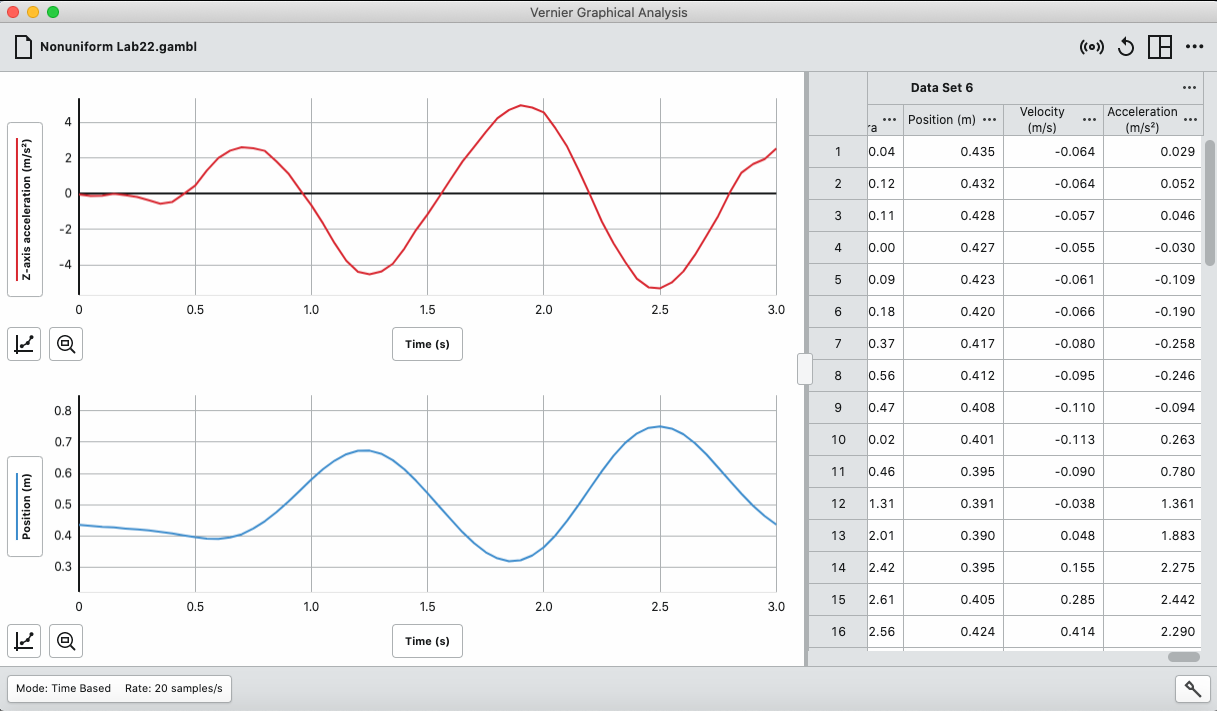
Using Graphical Analysis you will view and analyze the position data measured by the motion detector and the acceleration data measured by the accelerometer. The velocity of the object is calculated automatically with the default settings of the program, but you will also determine it twice more using calculus – once based on the position data and once based on the accelerometer data.
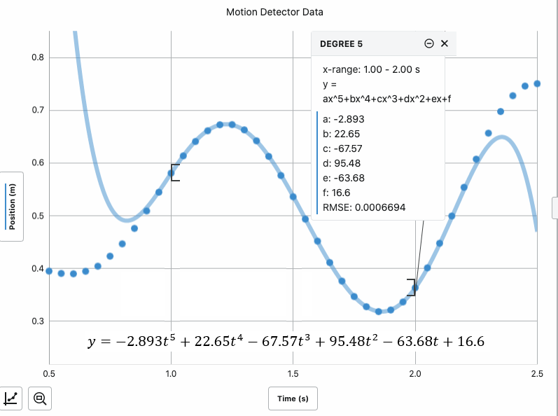
1. Inspect the graphs closely and find a particular interval of time (with roughly 10 to 20 data points) that includes a relative maximum or minimum of position and which shows a smooth curve in both the position and acceleration graphs (z-axis acceleration data from accelerometer). The goal is to find an interval of time that can yield nice curve fits in both graphs. Calculus will be applied to each curve fit to determine the velocity of the object for the same interval.
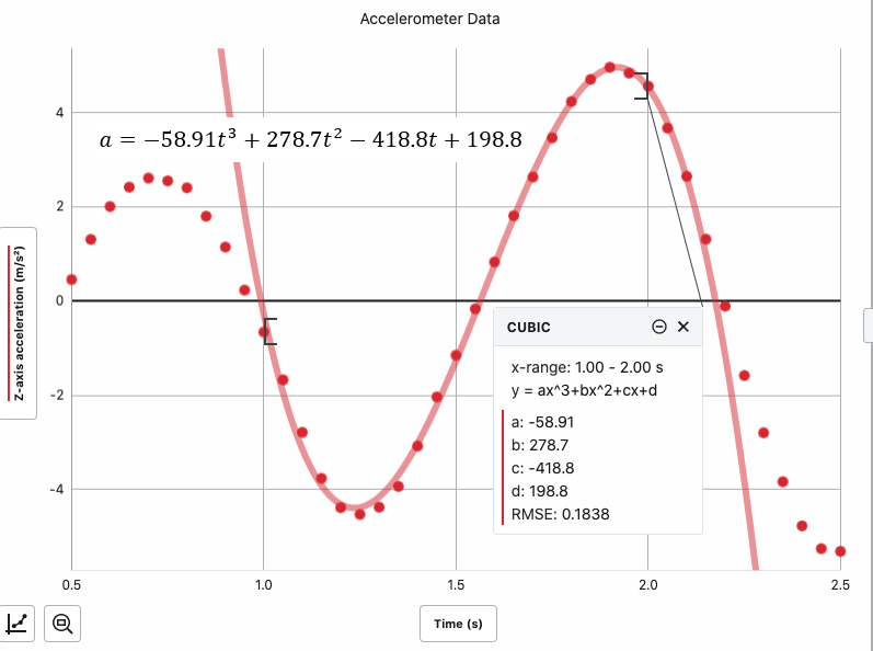
2. Insert automatic curve fits (Apply Curve Fit, Create Custom Fit…) on the exact same interval of time in both the position and acceleration graphs. Use an appropriate type of equation that will match the data well – polynomials are convenient for most situations. It is helpful to change the graph to show individual data point symbols without connecting lines. Then choose the same number of data points in the other graph corresponding to the same points in time. Note: use calculus to choose an appropriate set of curve fit equations – for example if the position graph has a quartic curve fit then the velocity graph would be cubic and the acceleration graph should have a quadratic curve fit based on the power rule for differentiation.
3. Determine the derivative of the curve fit from the position graph.
4. Determine the antiderivative of the curve fit from the acceleration graph. In order to determine the arbitrary constant, use a point in time at which the object reached a relative minimum or maximum in position (find this point by simply tracing along the position graph – you may want to use the “Interpolation” option). Based on this particular value of time you should be able to determine the value of the arbitrary constant. You will have to turn in a copy of the work showing how this was done.
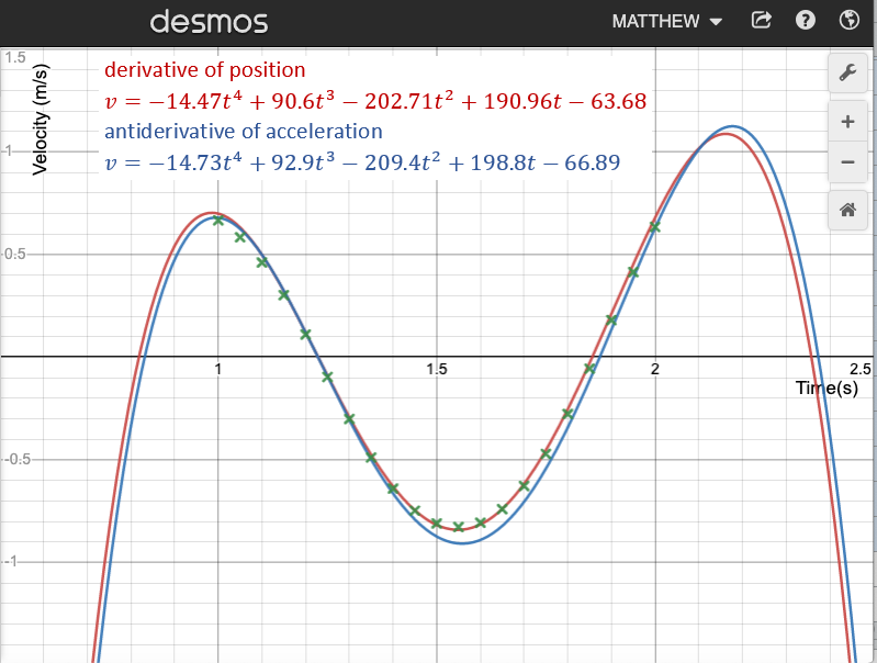
5. Use a program like Desmos to create a well-labeled and appropriately scaled graph of Velocity vs. Time showing the two curves found in the previous two steps. Also include on the same graph the discrete values for velocity from the automatic data table in Graphical Analysis (if you are using Desmos you can copy and paste data from the table). You should now have three determinations of velocity showing on one graph: derivative of position vs. time, antiderivative of acceleration vs. time and discrete approximations of velocity as calculated by Graphical Analysis using a numerical algorithm.
Printing tips and suggestions:
1. Adjust colors, point protectors, graph titles, labels, legends, fonts, etc. to produce the most informative and easy to interpret results possible. You can control the appearance of almost anything so you are responsible for the product! (Don’t blame computer for poor result.)
2. Export images of the graphs to an app or program suitable for printing, such as Microsoft Word or Google Docs. You can use screenshots or export images as separate files.
Questions
1. Discuss how well the results support the concepts that velocity is a derivative of position and acceleration is a derivative of velocity. Be specific and refer to the graphs, curves, equations, data, etc.
2. Show work and numerical calculations, detailing the steps that were taken, for determining the velocity function based on the automatic curve fit shown on the acceleration graph. In other words, show how you got the equation for the curve as described in Analysis step #4.
3. Using the curve fit equation from the acceleration graph, determine the maximum amount of jerk that occurred during the interval of time that was selected. Note that jerk is the time rate of change in acceleration. Use appropriate calculus techniques and show all work.
4. Discuss error. Of particular interest is the velocity that was determined thrice: as a column of values calculated automatically by the program (based on motion detector data), as a derivative of a curve fit on the position graph (motion detector data), and as an antiderivative on the acceleration graph (accelerometer data).
A complete report consists of the following (in this order):
o Summary page with data table and two graphs showing entire experiment
o Position vs. Time graph, with automatic curve fit
o Velocity vs. Time graph, with two curves and discrete points
o Acceleration vs. Time graph, with automatic curve fit
o Responses to questions 1 – 4, on separate paper.
Typical results: